The concept of the experience curve is also known as the degression effect and states that each time the quantity of a good is doubled, the unit costs can be reduced by around 20 to 30 percent. That sounds pretty promising, so in this post we took a closer look at how the experience curve works and what conclusions you can possibly draw from this concept for your company.
Experience curve – definition
The experience curve is a concept from the USA that says that the unit costs constantly decrease by 20-30 percent when the total amount of units produced doubles. The entire approach is based purely on the two factors of the total amount of products and the cost per piece .
In concrete terms, this means that companies that manage to increase their production volume many times over can expect significantly lower costs per unit. Those who manufacture significantly more products than competitors can produce at more favorable terms per item and thus either sell with higher margins or offer lower sales prices.
The concept of the experience curve
There are several conceivable reasons for passing the experience curve. In this context, there is often talk of “ economy of scale ”, that is to say of cost advantages that arise purely from increasing the quantity. In this context, scaling means that the costs per piece are reduced through mass production . Higher quantities enable the use of newer, better technologies. Let us think, for example, of the comparison of the manufacturing costs of hand-made products with machine-made goods, regardless of the type. The mass of products sold makes it possible to use a machine for automation to acquire or even to develop from scratch. This device reduces the costs per unit, the contribution margin increases or the sales volume is increased by reducing the price (which is possible thanks to the falling unit costs without sacrificing margins) and this creates a cycle that allows further cost reductions per unit.
Clearly, the experience curve is a curve with a flattening course . After all, at some point there are minimal costs that can hardly be reduced, because even highly automated and optimized processes come up against certain limits at some point.
Experience curve explained using the graphic
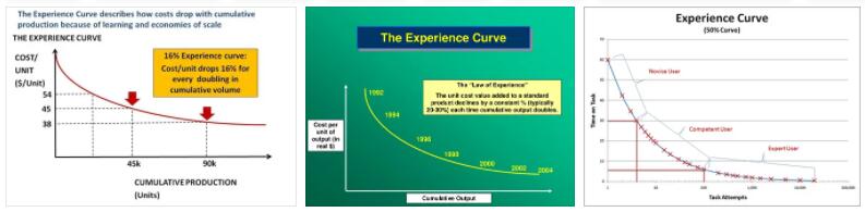
If you now look at the experience curve in the graphical representation, you will see at first glance that it is basically a simple basic idea. On the left we see the costs per piece and on the X-axis the cumulative quantity . If the amount is small, the unit costs are very high and the larger the output, the lower the unit costs. Ultimately, the effect is greatest at the beginning. At a later point in time, the course of the drawn line becomes flat again – so there is no further potential for optimization more available, even by increasing the quantity it is no longer possible to reduce the costs even further. This means that even with an extreme increase in the amount, costs are now only incurred that are de facto unavoidable.
The graphic clearly shows how the experience curve runs and what conclusions you can draw from it. If you manage to increase the amount of a product accordingly, you will be able to achieve corresponding savings. This can become a real competitive advantage , as they either generate a higher contribution margin or can offer them more cheaply than your competition.
Example and calculation
The easiest way to understand what is supposed to be gray theory is always using practical examples. So let’s imagine that a company produces goods and then sells them. By reducing the unit costs by 20 percent when doubling the output, the following scenario arises:
In the first year, a piece is first produced, the unit costs are 1,000 euros. Then two pieces are produced, the costs per piece are reduced by 20 percent (the output was doubled), so the costs per piece are only 800 euros. There is another increase, the company will produce four units in the next period. Based on the previous cost of 800 euros per unit, the costs are now reduced by a further 20 percent, so they are 640 euros per unit.
For the calculation it is therefore important to always determine the assumed reduction of 20 percent from the previously achieved cost value and not from the original starting value .
Compared to the production of a single piece as at the beginning, the unit costs could be reduced drastically. The example can now be continued until the point is reached in practice at which no further reductions are possible or these become marginal.
Causes of the degression
The question now also arises as to how it is possible that the unit costs can be reduced so much if the quantity of goods produced increases. The reasons can be different and if you want to find out for your own company, you should already pay close attention to where there are savings opportunities in the course of increasing the output volume. This will make you aware of the real potential and where the greatest savings were possible. You may be able to use this knowledge later if you also increase the production volume of other products.